Poor hand-to-mouth
Little liquidity and nonpositive net illiquid wealth.
An interactive research companion
Gold and Household Financial Constraints in India
A family can own a home, land or jewellery and still struggle to pay its bills. We study which wealth households can use—and how their spending responds when income changes.
Owning wealth does not make it ready to spend. A home provides shelter and gold stores value. Paying today’s bills requires cash, or a way to turn an asset into cash.
Gold can provide cash more quickly and with less paperwork than a home. Selling or borrowing against housing involves finding a buyer or lender, checking ownership documents and valuing the property. Both assets can be collateral, but they differ in how readily households can use them.
India has an established market for loans against gold. The World Gold Council describes this route to short-term finance. The Household Finance Committee documents gold’s broad acceptance as collateral and barriers to borrowing against real estate.
This distinction motivates our gold comparison. Later chapters ask how much potential liquidity gold provides and which housing assets belong in illiquid wealth.
We bring income and consumption together with assets and debts. The two surveys observe different parts of household finances; their common information lets us predict what each one is missing.
The Consumer Pyramids Household Survey follows household income and spending.
Common household
characteristics
The All-India Debt and Investment Survey records detailed assets and liabilities.
These are predictions across complementary surveys, not a record linkage of the same households. The paper harmonizes their common variables and evaluates predictions on held-out households.
Preferred approachGradient boosting is selected using total-income prediction performance; component targets can have a different best-fitting method.
| Method · click to learn more | R² · fit |
|---|---|
Gradient boostingPreferredGradient boosting builds trees sequentially to reduce prediction error. Income uses at most 500 iterations, learning rate 0.06 and early stopping. Wealth uses a two-part model: a positive-amount classifier with at most 400 iterations and a log-amount regressor with at most 500, both at learning rate 0.06. Wealth ownership thresholds are calibrated using training data; positive amounts use Duan smearing. | 0.810 |
Consumption-bin benchmarkThe consumption-bin benchmark splits the weighted training consumption distribution into 50 bins. Within each bin it estimates the ratio of mean consumption to mean income, then predicts income using household consumption and that ratio. No other household predictors enter. | 0.581 |
Consumption-rank mappingConsumption-rank mapping assigns each household the target value at the same weighted percentile as its consumption. The empirical mapping is fitted using training households. It preserves the target distribution but does not use demographic or financial predictors. | 0.543 |
Random forestRandom forest averages predictions across independently grown trees. The saved income and two-part wealth specifications use 300 trees, at least five observations per leaf, and 30% of predictor columns at each split. Wealth uses separate classifiers and positive log-amount regressions, with calibrated participation thresholds and Duan smearing. | 0.777 |
Gradient boosting · reweightedReweighted gradient boosting uses a classifier of survey membership to reweight CPHS toward AIDIS before fitting the income model. The survey probability is clipped to [0.001, 0.999] and converted to odds. The income regressor keeps the gradient-boosting settings: at most 500 iterations, learning rate 0.06 and early stopping. | 0.792 |
Elastic netElastic net fits a linear model with both absolute-value and squared-coefficient penalties. Income uses five-fold cross-validation over mixing values 0.1, 0.5, 0.9 and 1.0, with at most 5,000 solver iterations. The wealth ownership stage uses L1 logistic regression with C=1, the liblinear solver and at most 300 iterations; its positive log-amount stage uses the same five-fold mixing grid and at most 3,000 iterations, followed by Duan smearing. | 0.741 |
Gradient boosting · consumption measure 2This gradient-boosting specification replaces the standard consumption measure with alternative total consumption. The saved income alternative uses at most 250 iterations, learning rate 0.06 and early stopping; the two-part wealth alternative uses at most 200 iterations in each part, the same learning rate and early stopping. | 0.798 |
Gradient boosting · nondurable consumption 1This gradient-boosting specification replaces the standard consumption measure with nondurable consumption, definition 1. The saved income alternative uses at most 250 iterations, learning rate 0.06 and early stopping; the two-part wealth alternative uses at most 200 iterations in each part, the same learning rate and early stopping. | 0.801 |
Gradient boosting · nondurable consumption 2This gradient-boosting specification replaces the standard consumption measure with nondurable consumption, definition 2. The saved income alternative uses at most 250 iterations, learning rate 0.06 and early stopping; the two-part wealth alternative uses at most 200 iterations in each part, the same learning rate and early stopping. | 0.799 |
Gradient boosting · usual consumption expenditureThis gradient-boosting specification replaces the standard consumption measure with usual consumption expenditure. The saved income alternative uses at most 250 iterations, learning rate 0.06 and early stopping; the two-part wealth alternative uses at most 200 iterations in each part, the same learning rate and early stopping. | 0.787 |
Gradient boosting · self-production incomeThis gradient-boosting specification replaces the standard consumption measure with self-production income. The saved income alternative uses at most 250 iterations, learning rate 0.06 and early stopping; the two-part wealth alternative uses at most 200 iterations in each part, the same learning rate and early stopping. | 0.737 |
Gradient boosting · consumption excludedThis gradient-boosting robustness specification excludes consumption from the predictor set. Other income-model settings remain at most 500 iterations, learning rate 0.06 and early stopping, using the same testing households. | 0.737 |
Ordinary least squaresOrdinary least squares fits a linear relationship between transformed income and household predictors. Total income uses logs; other income targets use the inverse hyperbolic sine. The model uses survey weights and the common household testing split. It has no regularization parameter. | 0.722 |
OLS · consumption measure 2This OLS specification replaces the standard consumption predictor with alternative total consumption. It otherwise uses the same linear-model design and testing households as the OLS comparison; no regularization penalty is applied. | 0.715 |
OLS · nondurable consumption 1This OLS specification replaces the standard consumption predictor with nondurable consumption, definition 1. It otherwise uses the same linear-model design and testing households as the OLS comparison; no regularization penalty is applied. | 0.724 |
OLS · nondurable consumption 2This OLS specification replaces the standard consumption predictor with nondurable consumption, definition 2. It otherwise uses the same linear-model design and testing households as the OLS comparison; no regularization penalty is applied. | 0.717 |
OLS · usual consumptionThis OLS specification replaces the standard consumption predictor with usual consumption expenditure. It otherwise uses the same linear-model design and testing households as the OLS comparison; no regularization penalty is applied. | 0.684 |
OLS · self-productionThis OLS specification replaces the standard consumption predictor with self-production income. It otherwise uses the same linear-model design and testing households as the OLS comparison; no regularization penalty is applied. | 0.592 |
LassoLasso fits a linear income model with an absolute-value penalty that can set coefficients to zero. The saved Stata comparison chooses its penalty using five-fold cross-validation; the aggregate metrics workbook does not record the selected penalty. | 0.724 |
OLS · consumption excludedThis OLS robustness specification excludes consumption from the predictor set and keeps the same testing households as the income-model comparison. | 0.587 |
CPHS holds out 20% of households for testing; the current income metrics use 25,981 testing households. Models use the same saved split. Total-income errors are in logs; component-income errors use the inverse hyperbolic sine.
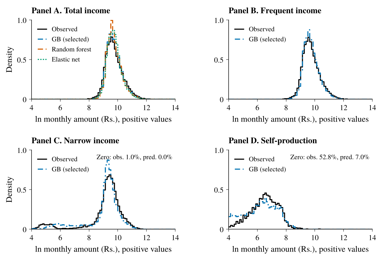
Saved survey-weighted CPHS testing histograms. Positive income is shown in natural-log rupees. Black: observed; blue: preferred gradient boosting; orange: random forest; green: elastic net where shown. Each panel retains its original positive-value sample.
Current prediction specifications describe age groups rather than the household head: counts below 18, at 18–24, at 25–64 and at 65+, men and median age among 25–64-year-olds, education, religion, caste, employment type, state and district. Financial predictors include consumption, livestock, tractors and cars, bank accounts, saving in shares and mutual funds, borrowing sources and purposes, and vehicle counts. Wealth models additionally include debt service. The headline excludes indicators identified as non-comparable across surveys, including house ownership, two-wheeler ownership, fixed deposits and gold saving. The older saved AIDIS characterization retains head-based demographics; a complete current predictor-by-HtM summary has not yet been exported.
The clickable method descriptions report the saved training and tuning choices. Figures show saved aggregate distributions; the website contains no household predictions.
Hand-to-mouth households have little liquid wealth relative to income. Some also have little net illiquid wealth; others own assets that do not readily pay for current spending. The distinction follows Kaplan, Violante and Weidner (2014).
A household living from paycheck to paycheck can still have cash on the day it is interviewed. If income arrives at the start of the month and is spent steadily, cash falls from the full paycheck to zero before the next payment. Its average balance over the month is half the paycheck.
That average gives us a benchmark for identifying limited liquidity. We compare survey balances with half of monthly income, following Kaplan, Violante and Weidner (2014, Section II). The survey balance is a snapshot within the payment cycle, so the rule approximates living hand to mouth; it does not observe each household’s spending path.
Halfway through: ₹5,000 in cash. The monthly average stays ₹5,000.
The implemented rule uses net liquid wealth: liquid assets minus liquid debts. For nonnegative balances, a household is hand-to-mouth when this is no more than half its monthly income. A larger balance places it in the non-hand-to-mouth group under this benchmark.
For borrowers, the rule measures remaining borrowing room. It assumes an unsecured credit limit equal to one month’s income and counts a borrower as hand-to-mouth when net liquid wealth plus that limit is no more than half monthly income. Negative net liquid wealth alone is not enough.
Illiquid wealth then separates poor from wealthy hand-to-mouth households. The gold options below change which resources enter each part of the balance sheet.
Little liquidity and nonpositive net illiquid wealth.
Little liquidity, but positive net wealth in illiquid assets.
Sufficient liquidity under the classification rule.
These descriptions explain the categories; they are not individual household records. “Poor” and “wealthy” describe balance-sheet groups here, not income ranks.
Observed income · predicted balance sheets
Observed balance sheets · predicted income
Gold-collateral capacity, with gold illiquid. Gold stays illiquid. Capacity is sufficient when net liquid wealth plus 75% of eligible gold exceeds half of monthly income, with no minimum gold holding. This measures potential capacity, not observed borrowing. Percentages are survey-weighted shares of all households. These comparisons precede the joint housing-quality and gold-capacity reclassification.
Gold changes the boundary between wealth and liquidity. Treating it as illiquid can move households from poor to wealthy hand-to-mouth; treating it as liquid can move them out of hand-to-mouth status. Potential borrowing against gold provides a third comparison.
Gold changes the balance sheet used for classification. Counting it as illiquid changes the poor–wealthy split; counting it as liquid can change the total hand-to-mouth share. Each bar shows survey-weighted percentages within its saved comparison.
Gold offers an established route from household wealth to short-term cash. The Household Finance Committee (2017, Sections 1.4 and 4.1) reports limited mortgage participation despite substantial housing wealth, alongside broad acceptance of gold as collateral.
Speed matters when an expense cannot wait. For example, State Bank of India’s gold-loan information says applications are normally sanctioned on the same day. This illustrates the accessibility of gold lending; a home’s reported market value does not by itself establish access to an equally quick loan.
The capacity comparison asks whether the amount is sufficient. Gold stays in illiquid wealth, while a specified fraction of its value is compared with the liquid shortfall. This measures potential borrowing capacity, rather than a household’s observed decision to borrow.
The preferred definition treats gold as illiquid and combines the ₹100,000 real-estate screen, at least two of three low-infrastructure markers, and a 75% pledgeable gold fraction with no minimum holding.
The new poor group includes the original poor, all low-infrastructure wealthy households, and high-infrastructure wealthy households without sufficient gold capacity. The new wealthy group contains only high-infrastructure households with sufficient capacity. Non-hand-to-mouth households remain separate.
Matching joint shares and consumption estimates are not yet available in the saved results. The completed comparisons above retain their own definitions and samples.
Household characteristics put the classifications in context. AIDIS profiles compare income, consumption, financial resources and demographics. CPHS profiles compare housing infrastructure across gold definitions; a separate earlier profile includes income, consumption and other characteristics.
Compare income and consumption, financial resources, and demographic characteristics within each group.
Gold excluded · original asset definition. Gold is excluded. Life-insurance sums assured are removed, and income is predicted using gradient boosting. These profiles use an earlier AIDIS sample, separate from the household-share comparison.
| Characteristic | Poor HtM | Wealthy HtM | Non-HtM |
|---|---|---|---|
| Monthly predicted income₹ per month | 14,468n = 8,172 | 16,129n = 57,269 | 18,546n = 50,996 |
| Monthly consumption₹ per month | 9,187n = 8,172 | 9,625n = 57,269 | 10,715n = 50,996 |
| Consumption / predicted incomeratio | 0.64n = 8,172 | 0.63n = 57,269 | 0.62n = 50,996 |
| Characteristic | Poor HtM | Wealthy HtM | Non-HtM |
|---|---|---|---|
| Owns a house% within group | 1.65%n = 8,172 | 94.63%n = 57,269 | 84.78%n = 50,996 |
| Owns the dwelling% within group | 1.59%n = 8,172 | 92.60%n = 57,269 | 82.98%n = 50,996 |
| Has a bank account% within group | 86.12%n = 8,172 | 97.13%n = 57,269 | 99.81%n = 50,996 |
| Has outstanding borrowing% within group | 25.21%n = 8,172 | 49.99%n = 57,269 | 31.94%n = 50,996 |
| Borrows from a moneylender% within group | 7.94%n = 8,172 | 15.46%n = 57,269 | 4.63%n = 50,996 |
| Monthly debt service₹ per month | 762n = 8,172 | 1,527n = 57,269 | 1,659n = 50,996 |
| Land area owned and possessedacres | 0.22n = 379 | 0.94n = 53,713 | 1.26n = 43,826 |
| Number of loanscount | 0.42n = 8,172 | 0.91n = 57,269 | 0.48n = 50,996 |
| Net liquid wealth₹ | -16,073n = 8,172 | -29,225n = 57,269 | 76,950n = 50,996 |
| Net illiquid wealth₹ | -20,731n = 8,172 | 1,471,045n = 57,269 | 2,421,214n = 50,996 |
| Liquid assets₹ | 3,144n = 8,172 | 5,502n = 57,269 | 78,835n = 50,996 |
| Illiquid assets₹ | 21,203n = 8,172 | 1,493,106n = 57,269 | 2,471,150n = 50,996 |
| Liquid debt₹ | 19,217n = 8,172 | 34,727n = 57,269 | 1,885n = 50,996 |
| Illiquid debt₹ | 41,934n = 8,172 | 22,061n = 57,269 | 49,936n = 50,996 |
| Land / illiquid assets% of assets | 32.83%n = 351 | 52.85%n = 57,269 | 56.50%n = 46,295 |
| Buildings / illiquid assets% of assets | 42.52%n = 351 | 43.09%n = 57,269 | 39.49%n = 46,295 |
| Provident funds and pensions / illiquid assets% of assets | 5.23%n = 351 | 1.65%n = 57,269 | 2.78%n = 46,295 |
| Other financial assets / illiquid assets% of assets | 19.43%n = 351 | 2.40%n = 57,269 | 1.23%n = 46,295 |
| Gold / (illiquid assets + gold), memo item% of assets | 97.09%n = 5,665 | 7.55%n = 57,269 | 13.94%n = 49,610 |
| Characteristic | Poor HtM | Wealthy HtM | Non-HtM |
|---|---|---|---|
| Age of household headyears | 36.82n = 8,172 | 48.48n = 57,269 | 48.85n = 50,996 |
| Household head: years of educationyears | 7.21n = 8,172 | 5.05n = 57,269 | 7.20n = 50,995 |
| Female household head% within group | 22.21%n = 8,172 | 12.87%n = 57,269 | 13.25%n = 50,996 |
| Household sizepeople | 3.02n = 8,172 | 4.55n = 57,269 | 4.26n = 50,996 |
| Members younger than 18people | 0.88n = 8,172 | 1.23n = 57,269 | 1.02n = 50,996 |
| Members aged 65 and olderpeople | 0.10n = 8,172 | 0.27n = 57,269 | 0.30n = 50,996 |
| Urban households% within group | 68.32%n = 8,172 | 25.12%n = 57,269 | 37.14%n = 50,996 |
| Caste: Scheduled tribe% within group | 8.74%n = 8,172 | 10.52%n = 57,269 | 9.48%n = 50,996 |
| Caste: Scheduled caste% within group | 21.01%n = 8,172 | 23.22%n = 57,269 | 14.45%n = 50,996 |
| Caste: Other backward class% within group | 43.80%n = 8,172 | 44.09%n = 57,269 | 42.84%n = 50,996 |
| Caste: Other caste% within group | 26.44%n = 8,172 | 22.18%n = 57,269 | 33.23%n = 50,996 |
| Religion: Hindu% within group | 78.42%n = 8,172 | 82.00%n = 57,269 | 83.26%n = 50,996 |
| Religion: Muslim% within group | 15.31%n = 8,172 | 12.43%n = 57,269 | 11.03%n = 50,996 |
| Religion: Christian% within group | 4.37%n = 8,172 | 2.95%n = 57,269 | 2.57%n = 50,996 |
| Religion: Sikh% within group | 1.06%n = 8,172 | 1.57%n = 57,269 | 1.82%n = 50,996 |
| Religion: Jain% within group | 0.23%n = 8,172 | 0.13%n = 57,269 | 0.35%n = 50,996 |
| Religion: Buddhist% within group | 0.49%n = 8,172 | 0.59%n = 57,269 | 0.65%n = 50,996 |
| Religion: Other religion% within group | 0.12%n = 8,172 | 0.32%n = 57,269 | 0.33%n = 50,996 |
Category percentages use weighted means. The mean/median control also applies to continuous portfolio ratios. Counts are specific to each variable where available; “—” means that statistic is not available.
This selection contains income and consumption, financial variables, demographics. Expand each table to see the available characteristics.
A temporary income setback and a lasting income change need not produce the same spending response. We separate these shocks and compare annual consumption responses across household balance sheets.
An elasticity of 0.20 means a 1% income change corresponds to a 0.20% consumption change in that exercise.
An MPC of 0.20 means a one-rupee income change corresponds to a 20-paise consumption change.
These are illustrative interpretations, not estimates. The explorer below reports each measure only when it is present in the saved results.
BPP · lagged consumption response · MA(1)
Points show estimates. Lines show ±1 saved standard error.
% change in consumption per 1% change in income
This annual comparison pools poor HtM households with wealthy HtM households without gold capacity. The household-share exhibit reports those two categories separately.
| Household group | Estimate | Standard error | Households |
|---|---|---|---|
| Poor + wealthy without gold capacity | 0.2108 | 0.0048 | 18,377 |
| Wealthy with gold capacity | 0.1867 | 0.0035 | 31,780 |
| Non-HtM | 0.2141 | 0.0024 | 72,674 |
Downloads retain source precision. The plotted lines are standard errors, not 95% confidence intervals. Saved unit conversions retain the precision of their source tables.
BPP fits income and consumption second moments by minimum distance. The selected lagged-response version allows the consumption response to a temporary shock to extend into the next period. Commault uses future income growth; the choice of lead is displayed. Crawley–Kuchler compares consumption and income changes at the selected change lengths.
The sample consists of households with a 2019 classification and at least one member aged 25–64. Income and consumption must be positive. Total consumption excludes self-production. Income and consumption are CPI-deflated and divided by the household’s mean real monthly income, excluding 2020 from that mean. Observations outside the calendar-month 1st–99th percentiles of either ratio are removed. This is the Crawley–Kuchler trimming rule used across the three methods.
Annual observations require at least eight of twelve months. First stages are fitted separately within each sample window. The full sample retains the COVID period and includes COVID interactions. Estimation is unweighted; the source supplies household-clustered uncertainty. Counts therefore differ from survey-weighted classification populations.
The preferred combined housing-screen, infrastructure and gold-capacity partition has no matching saved estimate. The available low-infrastructure and gold-capacity groups are separate comparisons. Rupee MPCs are displayed only when explicitly saved; no log coefficient is converted here.
The annual estimates describe income innovations inferred from the panel. Job loss offers a complementary view of a concrete household event.
We follow income and consumption around job loss and compare responses across household groups. The saved estimates connect the income change associated with job loss to the corresponding change in spending.
What counts as job loss? A previously employed wage worker is observed unemployed, willing to work and looking for work at the next interview, four months later. The comparison includes eligible workers who stay employed or are outside active job search.
Points show estimates. Lines show saved 95% confidence intervals.
₹ household consumption per ₹1 of worker wages
The IV estimate relates the change in household consumption to the change in the worker’s wages, using job loss as an instrument. It is a different exercise from annual BPP pass-through. Displayed n counts households; the sample can include more than one observation pair per household.
| Population | Estimate | 95% interval | Pairs | Job-loss pairs |
|---|---|---|---|---|
| All eligible workers | 0.1187 | 0.0738 to 0.1636 | 397,683 | 2,094 |
All eligible workers: first-stage F = 849.5; 97,926 households and 397,683 retained pairs.
Adjusted job-loss minus comparison differences, relative to each pair’s average in months −8 to −5. This pooled balanced sample is separate from the group comparisons above. The saved intervals are pointwise 95% confidence intervals.
97,735 households and 396,710 observation pairs, held fixed across all 13 months.
Constant-2014 rupees per month. The shaded span lies between interviews. These profiles are not MPCs, and the normalization does not establish parallel pre-trends.
Prior wage workers aged 25–62 are followed across interviews. The baseline retains zero consumption and zero wages. All eight financial months must be observed; the alternative sample requires positive consumption in every month. Total consumption excludes loan repayments and insurance premiums.
Interview windows sum the four months before the earlier interview and four months after the later interview, leaving out the intervening months. Calendar-wave comparisons instead use four-month means. Their timing and eligibility differ.
The unweighted two-stage least-squares model controls for age, age squared, sex, prior wages and state-by-endpoint-month effects (state-by-wave in the calendar-wave design). Uncertainty clusters by household. Groups use the fixed 2019 gold-illiquid classification, 75% pledgeable gold and no minimum holding. Group estimates require the later interview to be in January 2022 or after.
Pandemic windows from March 2020 through December 2021 are excluded. The sample retains repeated workers and concurrent household job losses; financial coverage ends in May 2025.
The research connects the composition of wealth to household financial constraints and consumption adjustment. Combining complementary surveys makes it possible to study those connections when no single survey observes every part of a household’s finances.
Gold and Household Financial Constraints in India
The paper develops the research question, methods and findings in full. This website lets you explore the latest aggregate results, including annual consumption responses and job-loss evidence. Each exhibit explains the definition and sample used for that comparison.
We welcome questions about the paper, feedback on the results and suggestions for this website. Mentioning a chapter or figure helps us find the comparison you have in mind.
Reach outEmail Aditi Singh at aditi.singh@cafral.org.in.
Gupta, Vivek, Fiorella Pizzolon, and Aditi Singh (2026). “When Is Wealth Liquid? Gold and Household Financial Constraints in India.” Working paper. https://papers.aditi-singh.com/India_HtM.pdf
Why households with substantial assets can still have little readily available wealth.
The framework for distinguishing consumption responses to permanent and transitory income shocks.
An alternative approach to estimating the response to temporary income changes.
A complementary way to compare consumption responses across household characteristics.
The wider setting for studying the composition of household balance sheets.
Institutional context for household portfolios and the role of gold in India.
This public release presents a fixed set of results. The figures and downloads use the same definitions and samples throughout.
The exhibits answer different questions about household finances. Household shares describe how common each group is, profiles describe the households within those groups, and consumption estimates describe responses to income changes.
Read each figure with its classification and sample. Shares use survey weights; consumption estimates use the sample and weighting stated in their section. A housing profile or an estimation sample can contain different households from the classification cross-section.
Elasticities and MPCs express responses in different units. Elasticities compare percentage changes; MPCs compare rupee changes. The charts label their uncertainty, and selections without a matching result show “Not yet available.”
You can download the aggregate data displayed in each exhibit. The download includes the group definitions, units and readable source labels, so the numbers can be interpreted alongside the paper.
The interactive controls could not load. The figures above remain readable. Please refresh the page to try again.